Exercise 2: Transform Data
In this exercise, you will clean and transform the data.
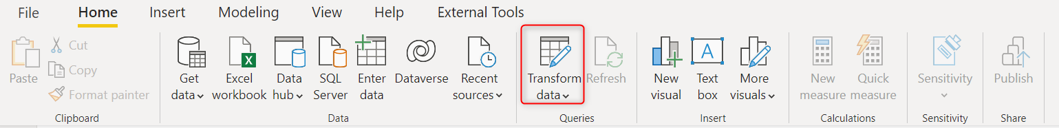
9. Select “Transform Data” on the top Ribbon. This will open Power Query Editor.
From here on you will use Queries and Tables interchangeably. Power Query shapes the data using code that is captured in a Query. The result of the Query’s output is a Table.
Queries: Queries and Steps
10. In Power Query you have queries on the left. Select the “2020 and Earlier Captures” query and then on the right-hand side take note of the Query Settings to see Properties and Applied Steps. Note that there are already applied steps. By default, when an Excel file is loaded, M code is automatically generated to load the data correctly and read the headers.
11. Now check the Crocs Query and notice the Column names are Colum1 and Column2.
The Crocs data doesn’t have column headers.
12. Under the Transform Ribbon, click Use First Row as Headers.
13. Note that on the right-hand side, in Applied Steps, the M code is updated with Promoted Headers.
14. Now check other queries to also make sure that they are picked up the column names correctly, and if not, go ahead and apply the first row as headers where needed.
Clean Zone Table: Transpose and Trim
15. The Zone data has column header but it’s not the right header. This is hard to work with when we want to filter by zones or create dynamic calculations about zones in our Power BI Desktop report.
16. On the right-hand side, notice the Applied Steps panel includes Promoted Headers and Changed Type. This is the way Power BI automatically detects pattern and data types, most of the time, it is correct but not always, this case is an example.
17. We would like to shape this query so that the columns are on rows, with 1 column called ZONE_NAME and another column of ZONE_CODE. On Applied Steps panel, delete Changed Type and Promoted Headers. We are going to switch to manual and reverse out these steps to unpivot the data. Notice the columns are now called Column 1, Column 2 etc and we have ZONE_NAME and ZONE_CODE as values under Column 1.
18. Under the Transform Ribbon, click Transpose to unpivot the columns to rows. Notice on the right, Transposed Table is applied and we now have two columns of data.
19. Promote the first row by clicking on Use First Row as Headers under the same ribbon.
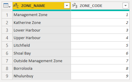
20. You notice that something still doesn’t look quite right about “Zone” data. Check the ZONE_NAME has a leading space in value for Management Zone. Can you clean this?
21. It is difficult to see how many spaces sometimes, but there is definitely at least one leading space here. Remove leading and trailing spaces in your data by selecting the column, right clicking, and selecting Transform -> Format – > Trim. Note that on the right-hand side, Applied Steps panel is showing “Trimmed Text”.
Captures Data: Add columns and Append
It’s easier to plot time trends and perform year-over-year calculations when all your historical captures data is one location – meaning one single Query. Before appending queries, for best practices, we also want to add an extra column. This can be extremely useful in case we need to trace data back to its source query later.
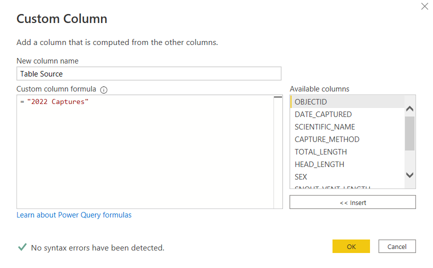
22. Click on “2022 Captures” > Custom Column. Give new column a name, for example “Table Source”. Under the box of “Custom column formula”, type “2022 Captures”. Click OK.
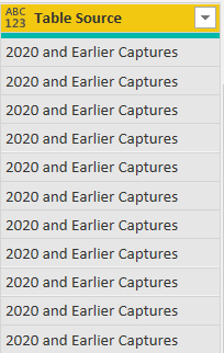
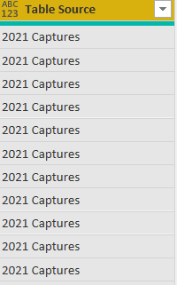
23. Now notice that on the very right-hand side of the query, there is a new column named Table Source with the content of “2022 Captures”.
24. Do the same for 2021 Captures and 2020 and Earlier Captures queries. Please note that the header “Table Source” must be exactly the same for 3 queries.

Now we do the append.
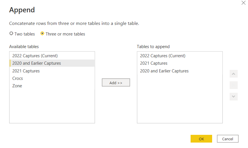
25. Click on “2022 Captures” > Go to the Home Tab > Select “Append Queries” towards the right of the ribbon > Check “Three or more tables”.

26. Add “2021 Captures”,”2020 and Earlier Captures” under “Tables to append” and select OK.
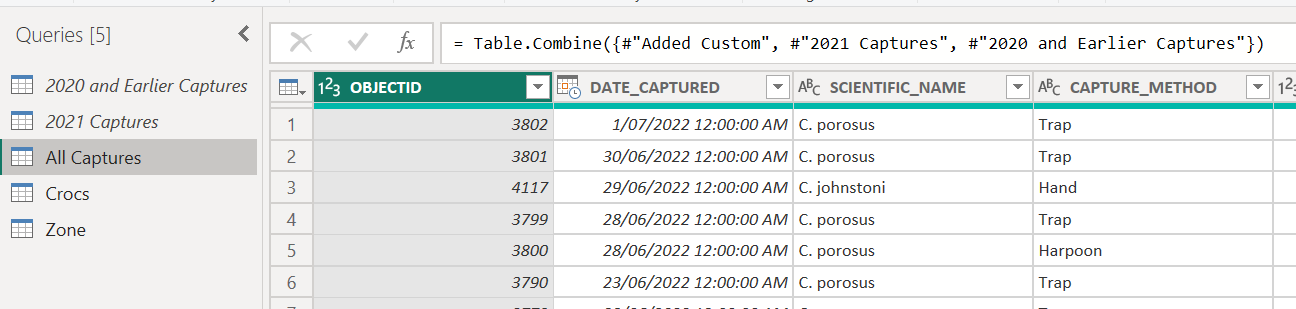
27. Ensure that you have all 3 datasets by clicking on the dropdown for Table Source and clicking “Load more”. You should see “2022 Captures”, “2021 Captures” & ”2020 and Earlier Captures” in the same data source.
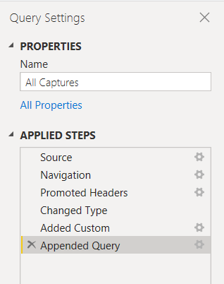
28. Rename the Query “All Captures”.
29. Now we have merged all 3 queries, we want to hide the single queries. To hide queries means they won’t load into the Power BI Report. On the left-hand side, right click on “2020 and Earlier Captures” and select “Enable Load” so that it is unchecked. Do the same for “2021 Captures”. Select “Continue” if a warning window pops up. There is no need to load the “2021 captures” and “2020 and Earlier Captures” into the report multiple times. All the information is all available in the new “All Captures” table. If you have done this correctly, you should see All Captures, Crocs and Zone and 2020 and 2021 queries will appear as italics.
Combine Crocs and All Captures Data: Join
30. Click on the “All Captures” query and look at the data. You see a column called “SCIENTIFIC NANME”, but click on the “Crocs” query and notice that it contains the “COMMON NAME”. We want to bring the common name into our “All Captures” query. Earlier you Appended two queries together to join them. We will now use a transformation called a Merge or Merge Queries. You notice that common names will be suitable for data analysis and dashboard user engagement. You decide to join them into your All Captures query.
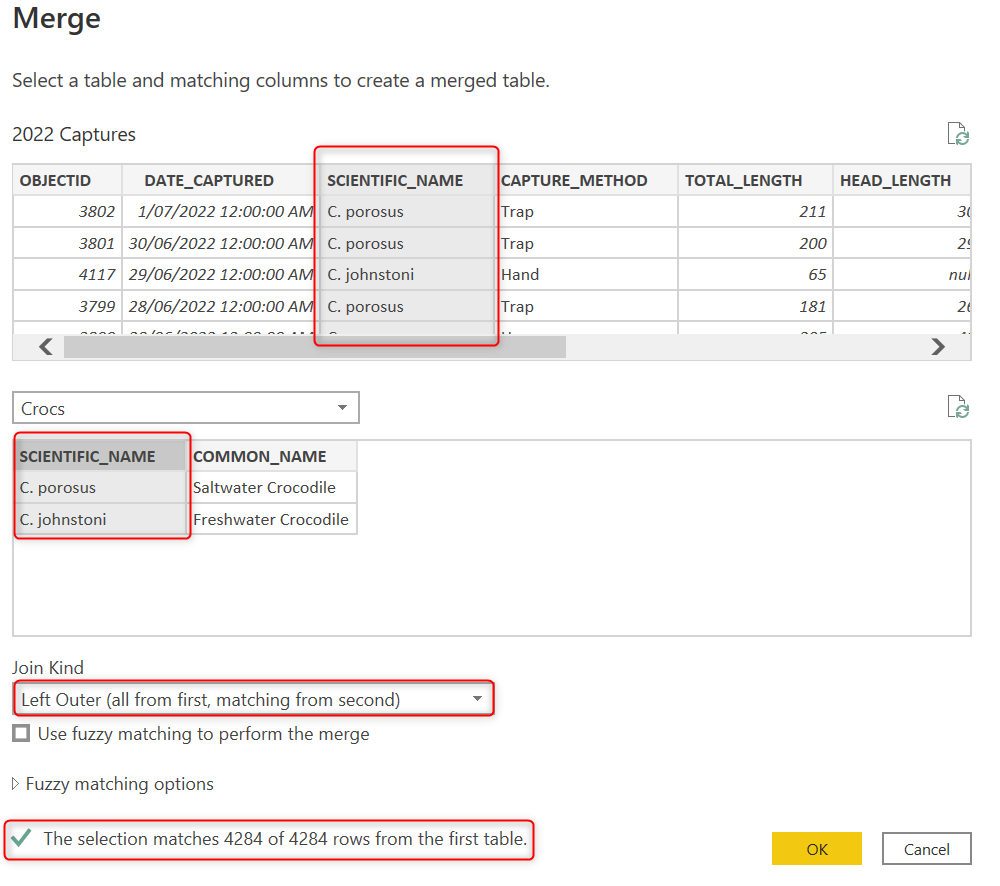
31. In “All Captures” table, go to Home > Merge Queries

32. Select SCIENTIFIC_NAME column in the “All Captures” table. Add a join to the Crocs table and select SCIENTIFIC_NAME as well. You should see a message at the end of the Merge screen which shows how many rows match between the two tables.
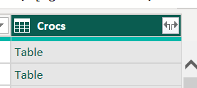
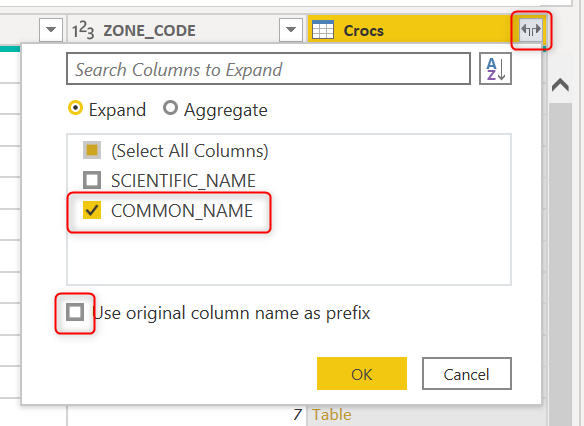
33. Once the tables are joined, we need to expand the Crocs table as all the fields from Crocs are in a single column. Click on the little icon at the top of the column with the top arrows going left and right.
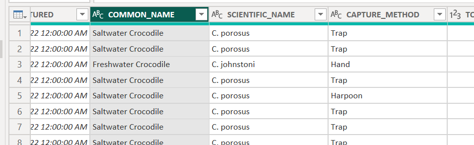
34. Add only the Common name we want by selecting the diverting arrows in the column header. Then make sure only “COMMON_NAME” is selected. Uncheck “Use original column name as prefix”.
35. You should now have a new column in your “All Captures” table but it is far over to the right. Move the COMMON_NAME next to SCIENTIFIC_NAME by clicking and dragging the column header for COMMON_NAME. Then delete SCIENTIFIC_NAME column by right clicking on the column > Remove.
36. Disable the Crocs table from loading into our Power BI report for now since all the information we need is included in the main table. Right click on the query and select Enable to disable.
Date Dimension: First steps to M language
Date Table is one of the most important dimensional tables using for calculating and operating time intelligence. There are several ways to create Date Table, so for simplicity and to demonstrate dates early in this course content, we will create Date Table in a very simply way – by loading dates from a text file. We will then be touching on some necessary first steps for consideration to getting your date table in the right shape within the Power Query functions and M code language.
40. Locate the “Date Table M Queries.txt” file within your Starter Materials. Open this file in Notepad and have a quick look. Do not worry, you will not write any code in there. Copy all of the code you see in this file. We will load this code to Power Query using a function. This Power Query function will generate a date table from scratch by specifying the start and end dates for your calendar.
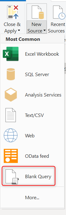
41. Open Power Query again by clicking Transform data. Select New Sources > Blank Query. Notice that Query1 appears on Queries panel.
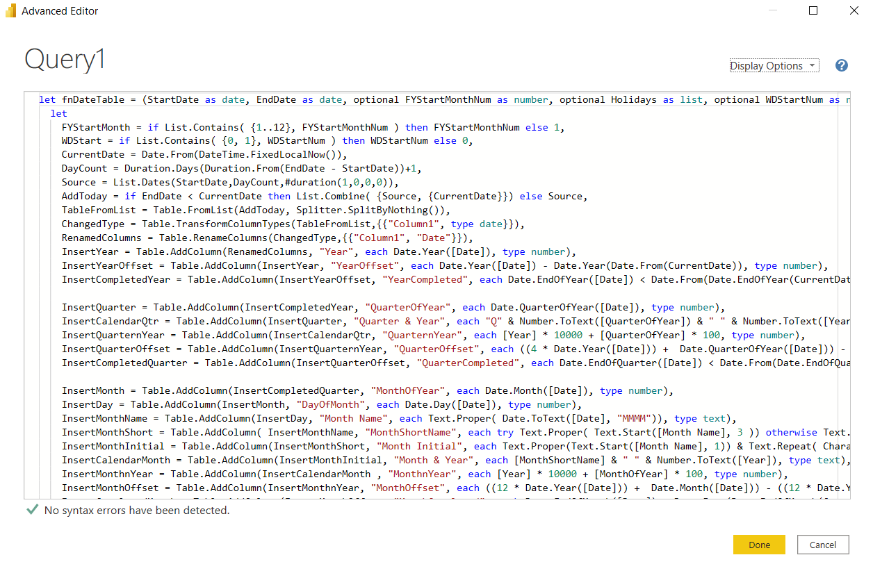
42. Go to Advanced Editor, this is a place where we start to write M code. Delete all the content in the window (there will by default be 4 lines with let and in) and copy the code in “Date Table M Queries.txt” file into the Query window.
43. Notice that No syntax errors have been detected. Hit Done.
44. Notice the icon next to your new Query shows fx. This query is generating a function where several inputs or Parameters can be entered to specify what dates you want in your date table. The Crocodile captures data includes captures from 1998 to 2022. Therefore, in the StartDate parameter value, enter 01/01/1998 and 31/12/2022 for EndDate. FYStartMonthNum presents the start month of financial year, skip it for now.
45. Select Invoke.
46. Notice on the left panel, the output of the Query has created a table named Invoked Function, and you also can see the a bunch of dates have been created starting with 1/01/1998 with a lot of columns describing all forms of that date. Rename “Invoked Function” to “Date Table”.
Set Relationships
47. As far as Power Query is concerned, it has just created Table called Date Table which has columns and data types. Click on the Date column, and notice in the Home ribbon under Data Type, that this column’s data type is Date. Click on the next column Year and notice it’s Data Type is a Whole Number. You should ideally set the data types for all of your data in the Power Query screen.
Hit “Close and Apply”. This closes the Query Editor and loads your changes into the Power BI Desktop and any reporting in that file.
48. Select the “Data Model” icon on the left-hand side.
49. Rearrange the tables so they look approximately like the picture below. If you are still seeing the Crocs table then go back to the Power Query editor and hide it.
50. In the next lab, we will delve into the world of Modelling, and will establish more relationships as well get your Date Table ready to work as a Time Machine.